Professional cable manufacturer

Professional cable manufacturer
Technical scope: steady-state cable current rating, thermal resistance, conductor losses and installation conditions. This article is aligned to the current IEC 60287 framework and is intended for engineering reference—not as a substitute for the applicable cable manufacturer's calculation or the governing installation code.
IEC 60287 is the IEC framework for calculating a cable's continuous current rating from its thermal circuit instead of looking it up in a table. The rating equation divides the permissible conductor temperature rise by the total thermal resistance of four paths — T1 through the insulation, T2 through the bedding, T3 through the serving and T4 through the external environment — and includes the dielectric and sheath losses. Because conductor AC resistance rises with temperature, the equation is solved iteratively. The core documents are IEC 60287-1-1:2023, IEC 60287-2-1:2023 and IEC 60287-3-1:2017, covering DC cables up to 5 kV.
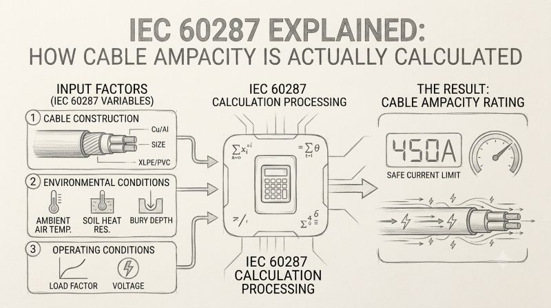
IEC 60287 is the IEC series for calculating the current rating of electric cables under steady-state conditions. The current core documents include IEC 60287-1-1:2023 for current-rating equations and losses, IEC 60287-2-1:2023 for thermal resistance, and IEC 60287-3-1:2017 for site reference conditions. IEC has also published additional Part 1 documents for specific loss and parallel-cable cases, including IEC 60287-1-2 and IEC 60287-1-3. IEC 60287-1-1:2023 and IEC 60287-2-1:2023 are the key references for the general calculation described here.
The IEC definition of steady state is important: the cable carries a continuous, constant current until the thermal condition approaches the maximum permitted conductor temperature, with the surrounding conditions treated as constant. IEC 60287-1-1:2023 applies to AC cables at all voltages and DC cables up to 5 kV, for cables installed directly in ground, in ducts, troughs or steel pipes, and in air. IEC official scope.
The basic engineering model is a thermal circuit. Electrical losses generate heat; thermal resistance determines how much temperature rise is produced for a given heat flow.
For a power cable, the dominant heat source is normally conductor loss, but metallic sheath/screen loss, armour loss and dielectric loss can also contribute. The relative importance depends strongly on cable construction, conductor size, voltage, bonding arrangement, frequency and installation.
For the standard thermal model used in the general steady-state equation, the heat path is represented by four thermal-resistance terms. Their exact calculation depends on the cable construction and installation geometry; the values should not be replaced by generic “typical” numbers when a project calculation is being performed.
Thermal resistance between the conductor and the metallic sheath/screen. It is primarily determined by insulation geometry and thermal properties.
Thermal resistance associated with the bedding or layer between metallic sheath/screen and armour, where applicable.
Thermal resistance of the external serving/sheath covering outside the armour or metallic layer, depending on cable construction.
External thermal resistance between the cable surface and the surrounding medium. For buried cables, soil properties and geometry are critical.
IEC 60287-2-1:2023 provides the calculation of thermal resistance for the relevant steady-state installation arrangements and also recognises cases where analytical methods are not sufficient and numerical methods such as finite-element methods may be needed for external thermal resistance. IEC 60287-2-1:2023.
Joule heating in the conductor. For AC calculations, the conductor resistance includes the effects represented by the IEC AC-resistance calculation.
Losses in metallic sheaths or screens caused by induced and/or circulating currents, depending on bonding and cable arrangement.
Losses associated with armour, reinforcement or relevant magnetic metallic components. The magnitude depends on construction and operating conditions.
Loss in the insulation under AC operation. It can be negligible for many LV applications but becomes relevant for higher-voltage cables.
The important point is that there is no reliable universal percentage such as “conductor loss is always 85–95% of total heat” or “armour loss is always 5–15%”. Those percentages depend on cable design and installation. They have therefore been removed from this revised version.
For AC cable calculations, the conductor resistance used by the IEC model is the AC resistance at the relevant conductor temperature. In general form, IEC 60287 represents it as the temperature-adjusted DC resistance modified by skin and proximity effects:
For copper, a commonly used temperature coefficient at 20 °C is approximately 0.00393 K−1. As temperature rises, conductor resistance increases. Skin and proximity effects can further increase AC resistance, particularly for larger conductors and certain cable arrangements.
For the common steady-state AC case without the special partial-drying or solar-radiation modifications, the general current-rating equation can be written as follows:
This equation is a compact representation of the standard model. The exact applicable equation must be selected according to the installation condition and the cable construction. IEC 60287-1-1:2023 includes separate treatments for buried cables with partial drying-out, conditions where drying-out is to be avoided, and cables directly exposed to solar radiation. IEC 60287-1-1:2023.
| Symbol | Meaning | Engineering note |
|---|---|---|
| Δθ | Permitted conductor temperature rise above ambient | Determined from the maximum permitted conductor temperature and the relevant ambient condition. |
| R | AC conductor resistance at the relevant temperature | Includes temperature effect and, for AC, skin/proximity effects as applicable. |
| Wd | Dielectric loss per unit length | Important mainly where dielectric losses are not negligible. |
| n | Number of load-carrying conductors | Must match the cable arrangement and the assumptions of the applicable equation. |
| λ1 | Sheath/screen loss factor | Depends on cable construction, bonding, geometry and frequency. |
| λ2 | Armour/reinforcement loss factor | Depends on armour construction and magnetic/electrical conditions. |
| T1–T4 | Thermal resistances | Calculated from cable construction and installation conditions. |
The resistance depends on conductor temperature, while the conductor temperature depends on the losses generated by current. This creates a temperature–resistance feedback loop.
The practical lesson is simple: a calculator that inserts a fixed resistance and never checks conductor temperature is not equivalent to a complete IEC 60287 rating calculation.
For buried cables, the external thermal environment can dominate the result. Soil thermal resistivity is commonly expressed in K·m/W. A higher resistivity means poorer heat transfer through the soil and therefore a lower permissible current, all else being equal.
IEC 60287-3-1:2017 defines site reference conditions for steady-state cable operation, but it explicitly notes that national requirements can supersede the general reference values. IEC 60287-3-1:2017.
Heat is removed more effectively from the cable environment, generally supporting a higher steady-state rating.
Heat removal becomes more difficult and the permissible current generally decreases.
For some buried installations, soil moisture migration and partial drying-out require the specific IEC treatment rather than a simple fixed-resistivity assumption.
Soil resistivity measurement, thermal backfill selection and burial depth are treated step by step in our direct-burial soil resistivity guide, and the ambient-temperature, grouping and altitude correction factors that stack on top of a base rating in our ampacity derating factors guide.
The earlier draft stated that a 120 mm² 4-core Cu/XLPE/SWA/PVC cable buried at 1 m in soil with ρ = 1.0 K·m/W had an “exact BS 7671 result” of 180 A. That statement has been removed.
The reason is important: BS 7671 table values are tied to their defined reference installation conditions and correction-factor system. They are not interchangeable with an arbitrary IEC 60287 scenario. The IET's current BS 7671 materials identify Appendix 4 as the section covering current-carrying capacity and voltage drop, with separate factors for ambient temperature, ground temperature, soil resistivity, burial depth and grouping. IET Appendix 4 reference.
Also note that, as of 2026, the current UK wiring regulation is BS 7671:2018+A4:2026, although a transition period allows work to continue under the previous edition until 15 October 2026. Therefore, any article quoting a BS 7671 table number should state the edition and should not mix an older table value with a modern IEC 60287 installation scenario. IET edition status.
IEC 60287 does not simply ignore solar heating. IEC 60287-1-1 includes specific rating equations for cables directly exposed to solar radiation, and the associated external thermal-resistance treatment is referenced to IEC 60287-2-1.
For outdoor PV and other exposed installations, the thermal calculation should therefore consider the actual installation environment, cable surface properties, solar radiation and the applicable conductor temperature limit. A simple buried-cable equation should not be reused unchanged for an exposed cable.
IEC 60287-1-1:2023 explicitly covers DC cables up to 5 kV under steady-state conditions. Therefore, a 1500 V DC cable is within the stated voltage scope of the standard. The DC formulation is simplified because AC-only effects such as skin and proximity effects do not apply in the same way to steady DC, and dielectric loss is not treated as an AC loss term.
However, a PV installation may be exposed to solar radiation and elevated ambient temperatures. The correct calculation must therefore match the actual installation condition rather than simply applying the buried-cable DC simplification. For the complete DC sizing workflow — voltage-drop limits alongside ampacity charts for 600 V and 1500 V PV strings — see our DC cable sizing guide for solar PV.
Harmonic currents can increase heating because conductor AC resistance and metallic-screen/sheath losses are frequency-dependent. The correct treatment depends on cable construction, harmonic spectrum, bonding arrangement and the applicable IEC calculation.
The previous article stated that “THD > 15%” could reduce ampacity by “10–20%”. That numerical rule has been removed because it is not a general IEC 60287 rule. For a real harmonic-rich installation, the harmonic current spectrum should be evaluated and the additional losses calculated appropriately.
IEC 60287 and the Neher–McGrath method both address the thermal problem of cable current rating, but they should not be described as producing “automatically similar” results or as being interchangeable. Each method has its own equations, assumptions, reference conditions and treatment of installation geometry.
For projects governed by NEC, use the applicable NEC tables and calculation provisions. For projects based on IEC methods, use IEC 60287 and the applicable national implementation. When comparing results, match the cable construction, ambient conditions, soil properties, spacing, burial depth, loading and other assumptions before drawing conclusions.
IEC 60287 is powerful, but a one-dimensional analytical model should not be treated as a universal solution for every thermal problem. Complex installations can require more detailed modelling.
IEC 60287-2-1:2023 explicitly includes reference to finite-element methods where analytical methods are not available for the required external thermal-resistance calculation. For cyclic and emergency current ratings, the IEC 60853 series is the relevant family of standards rather than IEC 60287 alone. IEC 60287-2-1 background and IEC 60853-2 reference.
Before starting a project-specific IEC 60287 calculation, collect the following information:
For a quick screening estimate before the full project calculation, the Sorivo online cable ampacity calculator applies the table-based method with ambient and grouping corrections. Use it to narrow the candidate conductor size, then confirm the final rating with the IEC 60287 calculation for your actual installation conditions.
Reference policy: standard numbers and scopes have been checked against IEC and IET material available at the time of revision. Exact project calculations should use the licensed/current edition of the applicable standard and manufacturer-specific cable construction data.
Need a project-specific cable rating? Sorivo can provide a calculation sheet based on your cable construction and installation conditions. Contact Sorivo engineering with conductor size, cable construction, installation method, ambient/ground conditions, spacing, burial depth and load information. Prefer a formal quotation? Ask a Quote.

How this was written: every figure in this article is checked against the standard or regulation listed in Sources before publication. Where a value is our own measurement, it is labelled as such.